MindshaRE: Using Binary Ninja API to Detect Potential Use-After-Free Vulnerabilities  – Zero Day Initiative – Blog

Use-after-free is a memory corruption condition where a program references memory after it has been released back to the allocator. Statically detecting these bugs can be challenging. In the past, several approaches have addressed this problem, such as GUEB by Josselin Feist and Sean Heelan’s work on Finding use-after-free bugs with static analysis.

This blog post explores the usage of Binary Ninja’s Medium Level Intermediate Language (MLIL) to establish a data flow graph by tracing interactions between a specific memory allocation and other memory regions. Building on the data flow graph, it is further utilized in context-insensitive reachability analysis across functions to identify potential Use-After-Free (UAF) vulnerabilities in binaries. Like any other static code analysis approach, this one also has classification errors. While acknowledging the classification errors inherent to static code analysis, we highlight primitives that may also be adaptable for modeling other types of vulnerabilities.

For readers interested in Binary Ninja APIs, refer to our earlier blog post, which comprehensively explains using Binary Ninja Intermediate Languages (ILs) and Static Single Assignment (SSA) form.

Building a Data Flow Graph of Memory Allocation

In this context, data refers to the pointer associated with a specific memory allocation that is the subject of tracking and analysis. The data flow information is visualized as a graph, where:

•    Nodes represent different memory regions.
•    Edges represent pointer store operations that establish relationships or interactions between these regions.

In this implementation, four distinct types of nodes are utilized to construct the data flow graph, each serving a specific purpose:

Tracked Allocation Node (Red): Represents a memory allocation of interest, and acts as the focal point for tracking interactions across the graph.

Function Stack Frame Nodes (Green): Represent the stack frames of individual functions visited during inter-procedural analysis.

Dynamic Memory Nodes (Blue): Represent Static Single Assignment (SSA) variables that cannot be tied to a specific source. These could include dynamically allocated memory or arguments passed to functions for which we lack insights within the scope of the function.

Global Memory Nodes (Black): Global variables across functions are not comprehensively tracked. However, these nodes help analyze interactions within a single function.

The edges in the graph represent pointer store operations, establishing connections between memory allocations. The source node corresponds to the memory being written to and the destination node represents the pointer value being stored. The edge attributes capture the offsets from allocation base addresses. The “write” attribute indicates the offset from the base of an allocation (source node) where the pointer is written to, and the “points” attribute indicates the offset within an allocation (destination node) that the written pointer value points to. New edges are created for every unique value of “write” or “points” attribute. Write operations to stack memory are represented using absolute values from the base of the stack as represented by Binary Ninja and hence will have negative offsets for most of the architectures. When “write” or “points” attribute is 0, it means base of an allocation. Edges are additionally created during unresolved memory load operations, assuming that the relevant memory store occurred outside the function scope. This graphical representation helps understand how memory regions interact. Below is a section of a sample graph generated during analysis of OpenSLP, providing better clarity on the details described:

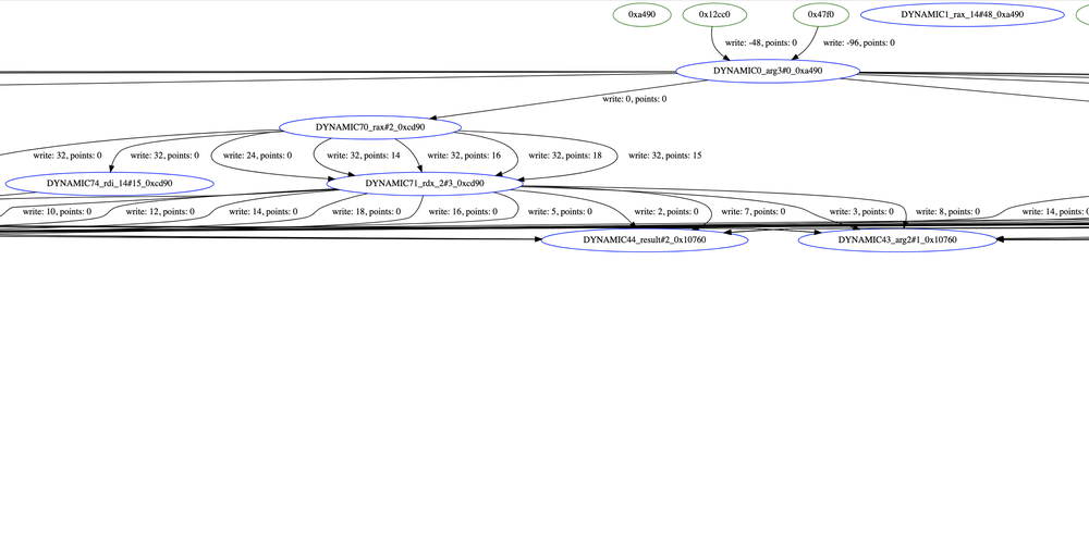
Mapping Relationships Between SSA Variables, Graph Nodes, and Edges

Now that we have an understanding of our graph structure, let’s explore how SSA variables are mapped to the nodes in the data flow graph. In our automated analysis, the first SSA variable to be tracked is the one assigned the return value of an allocator call, such as malloc() or calloc(). Furthermore, a Binary Ninja GUI interface could be developed to enable users to mark arbitrary variables for tracking and include them in further analysis. Once we identify the SSA variable of interest, we can leverage the definition-use chain to traverse all its uses within the function. Binary Ninja provides the get_ssa_var_definition() and get_ssa_var_uses() APIs to retrieve a variable’s definition site and its uses, respectively. Consider the below C code and Binary Ninja’s MLIL SSA representation of the same:

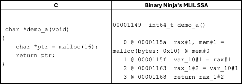
Here, the return value of call to malloc() is written to SSA variable rax#1 and the further usage of rax#1 in the function can be fetched using get_ssa_var_uses() API:

A variable points to a node, and in this context, rax#1 points to the Tracked Allocation Node (Red). When rax#1 is assigned to var_10#1, this information is propagated to var_10#1 and subsequently to any further assignments. When a variable assignment involves pointer arithmetic, a piece of offset information is stored in addition to the node. In this case, the offset is 0 because all the variables point to the base of the Tracked Allocation Node.

The ptr variable in the function stack is represented by the SSA variable var_10#1, which stores the pointer to the allocated memory. The offset for this variable can be extracted and represented as an edge in the graph. In essence, two data structures are constructed: a dictionary that maps SSA variables to nodes and a graph that connects various memory regions, represented as nodes. Since SSA variables are associated with their specific functions, they can be uniquely identified across functions during inter-procedural analysis.

The following code snippet demonstrates the creation of a Tracked Allocation Node (Red node) and the initialization of the SSA variable dictionary, which contains information about the SSA variable and the node it references:

Let’s examine another example of code and its MLIL translation to understand the process of creating a Dynamic Memory Node (Blue).

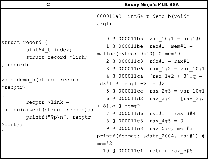
Within the function scope, there is no information about the location recptr points to. When recptr->link is initialized with the return value of a call to malloc(), a Dynamic Memory Node is created with an edge to the Tracked Allocation Node. This corresponds to the MLIL instruction 0000118a [rax_1#2 + 8].q = rdx#1 @ mem#1 -> mem#2 (MLIL_STORE_SSA), where the edge attribute contains the offset information. The variable rax_1#2 can be tracked back to arg1#0 using the SSA use-def chain.

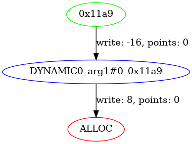
Essentially, whenever memory store operations such as MLIL_SET_VAR_SSA, MLIL_STORE_SSA, or MLIL_STORE_STRUCT_SSA are encountered, edges are created in the graph. In Binary Ninja’s MLIL SSA form, MLIL_SET_VAR_SSA is not strictly a memory store operation since stack writes are translated to SSA variables. However, the variables still retain offset information, which can be used to construct the data flow graph.

Translating Memory Loads to Graph Edges

While memory store operations are translated into graph edges, as previously discussed, load operations from memory outside the function scope are also represented as graph edges. Consider the following example:

Within the function scope, there is no specific information about recptr. However, when the pointer returned by malloc() is written to recptr_new->link, this memory is traced back to the argument passed, i.e., recptr (arg1#0), using the SSA use-def chain. The memory load operation recptr->link is translated to 0000117d rax_1#2 = [rax#1 + 8].q @ mem#0 in the MLIL SSA representation. This load operation is represented as an edge between arg1#0 and rax_1#2. The underlying assumption here is that if the memory is being loaded, it must have been initialized beforehand. Memory store, assignment, and load operations serve as the fundamental building blocks of the data flow graph.

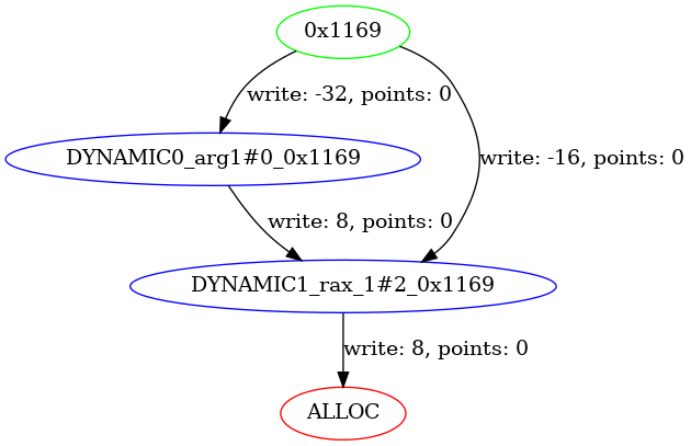
Traversing the Data Flow Graph to Propagate Information

Now that we understand how variables are initialized as mappings to nodes in the graph and how memory accesses are translated to edges, the next question is: how is this information propagated when traversing instructions in the SSA def-use chain? The answer lies in the SSA variable dictionary and the graph that we initialized previously.

        — A direct variable assignment is straightforward. The value of the source variable is assigned to the destination variable. Consider an expression like rax#0 = rbx#0. Here rax#0 is assigned with the value of rbx#0 from the SSA variable dictionary.

        — For a variable assignment where pointer arithmetic is involved, offset information is stored in addition to the node. Consider an expression like rax#0 = rbx#0 + 0x10. Here rax#0 is assigned with the node pointed to by source variable rbx#0 and holds the offset value to the node, which is 0x10.

        — For a variable assignment where pointer arithmetic is involved, the node information from the source variable is directly assigned to the destination variable, just as in the case of direct assignment. However, in this situation, the offset information is updated to reflect the pointer arithmetic operation. Consider an expression like rax#0 = rbx#0 + 0x10. Here rax#0 is assigned with the node pointed to by source variable rbx#0 but the offset value is set to 16.

        — A variable assignment where data is loaded from memory like rax_1#2 = [rax#1 + 8].q, the edges of the graph are visited to fetch the target node pointed to by the source variable. To detail further, the node and the offset associated with rax#1 (base variable) is fetched from the SSA variable dictionary. Then the final offset is computed as the sum of “offset” fetched from SSA variable dictionary and the offset from the load instruction. Once the node and the computed offset are available, we find the edge which has the “write” offset equal to that of the computed offset by walking through all the edges of the node. The destination node and “points” offset associated with this edge are assigned to rax_1#2. Essentially, we resolve a memory load operation to node and offset values, which can be used to update the SSA variable dictionary. Below is the code snippet to demonstrate this:

Callees are visited after all the instructions in a def-use chain of the calling function have been processed. A callee is considered for further analysis only if any arguments passed to the function have mappings in the SSA variable dictionary. Recursion is managed by monitoring the call stack for repeated calls to the same function and terminating the analysis after a predefined number of iterations.

In cases where stack memory is passed as an argument, the callee is also analyzed if the stack offset passed is less than the write offset value of any edges associated with the respective Function Stack Frame Nodes (Green). This consideration ensures that even if a structure element is initialized within a function and the base of the structure is passed to the callee (with the stack growing downwards and using negative offsets), the analysis accounts for it appropriately.

Once the instructions in the SSA def-use chains of both the caller and callees have been traversed, the data flow graph generation is considered complete, with all variable information fully populated for further analysis.

Logging Instructions Linked to Tracked Allocation

After completing the SSA variable mapping and generating the data flow graph, the instructions are revisited. All memory loads, memory stores, or call instructions dependent on the Tracked Allocation Node are recorded, along with the statically generated call stack. These are considered as “Use”. Additionally, call instructions involving deallocator functions are logged and considered as “Free”. Below is a sample code snippet for handling MLIL_STORE_SSA instruction:

Inter-Procedural Analysis for Use-After-Free Detection via Call Stack

Once the logging is done, detecting potential use-after-free bugs involves analyzing all basic blocks categorized as “Free” and verifying if any paths lead to basic blocks categorized as “Use”. If such a path exists, it is flagged as a potential use-after-free condition. Since double-free bugs are related to use-after-free, the analysis also examines whether a path exists from one “Free” block to another “Free” block. If such a path is detected, it is flagged and logged as a potential double-free condition.

In forward data flow analysis, there is at least one common function in the call stack leading to “Free” and the call stack leading to “Use.” For example, consider a scenario where function A allocates memory, passes it to function B for use, which propagates it further to function C, where it gets freed. The instructions using the allocation in B have a call stack of A leading to B, while the call stack for function C includes A leading to B and B leading to C. The last common function in these two call stacks is B.

The analysis conducted here is not context-sensitive and focuses solely on reachability. Therefore, instead of identifying a direct path between the basic block in C that frees the memory and the instructions in B that use the memory, the analysis checks for a path within the last common function, i.e., between the basic block in B that calls function C and the basic blocks in B that use the memory. This approach allows for inter-procedural analysis while limiting the pathfinding to the last common function, improving efficiency and scope control. Otherwise, one may have to inline multiple functions into a single graph to perform reachability analysis.

Additionally, loops require special attention to minimize false positives. In loops, backward edges can connect basic blocks following a deallocation to those preceding an allocation. Therefore, instructions executed after an allocation but before a deallocation can still appear reachable in the graph, potentially being misidentified as use-after-free. To mitigate this, all incoming edges to the basic block that invokes the allocator function are removed in the control flow graph. This effectively disconnects statements that would otherwise appear reachable within the loop, reducing the false positive results.

Automated Detection of Allocator and Deallocator Calls

While it is ideal to use allocator and deallocator wrappers specific to the program as input for this analysis, manually identifying them can be challenging. An easier starting point is to input standard functions like malloc(), realloc(), and free(), examine the outcomes, and progressively refine the analysis based on the results. By cross-referencing allocator functions like malloc() and leveraging def-use chains, we can determine if the pointer returned by an allocator function is subsequently returned by the caller. If so, the caller is likely a wrapper around the allocator. For finding deallocator functions, the approach is similar to the one mentioned as “Function aliases” by Sean Heelan. Binary Ninja’s dataflow analysis can be used to verify whether any of the caller’s function parameters are directly passed to a deallocator such as free(). This can be identified by checking if the parameter’s value type is RegisterValueType.EntryValue. If this condition is met, it indicates a potential wrapper around the deallocator function.

Using a JSON file with minimal allocator details, numerous functions involved in allocating and deallocating data structures were identified in OpenSLP. These discovered functions can be incorporated into the JSON file for further analysis. Currently, the “arg” key holds no significance in the implementation.

Since we perform forward data flow analysis, which involves visiting the functions that invoke the allocator call as well as the callees of those functions, identifying these wrappers allows us to shift the starting point of our analysis. Simply put, instead of beginning our analysis inside SLPMessageAlloc(), where forward data flow analysis has limited scope because it calls calloc() without further interactions, we can focus on analyzing all the functions that call SLPMessageAlloc(). This approach broadens the scope and provides better insights into the data flow.

Analyzing Real-World Vulnerabilities from the Past

To understand how the tool works, let’s test it on some known vulnerable programs. Since GUEB already provides a list of identified vulnerabilities, I chose to use them as examples here.

CVE-2015-5221: JasPer JPEG-2000

There is a use-after-free/double-free vulnerability in mif_process_cmpt() as seen in RedHat Bugzilla.

By tracking the allocation and deallocation APIs, jas_tvparser_create() and jas_tvparser_destroy() respectively, the following results are observed:

In this case, mif_process_cmpt() is inlined into mif_hdr_get(), and the results are displayed accordingly.

CVE-2016-3177: Giflib

Here is a double-free vulnerability in gifcolor – #83 Use-after-free / Double-Free in gifcolor

In this case, the allocation and deallocation APIs used were EGifOpenFileHandle() and EGifCloseFile(), respectively, and the results are as follows:

GNOME-Nettool

This use-after-free vulnerability in get_nic_information() – Bug 753184. For this analysis, g_malloc0() and free() pair is tracked:

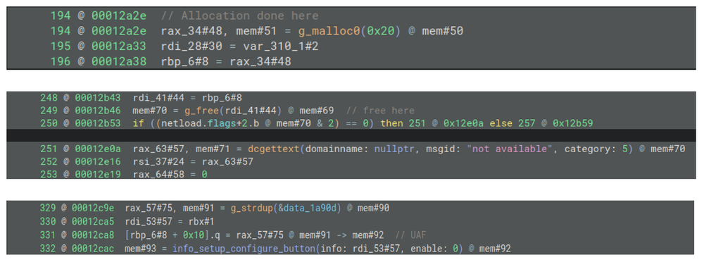
CVE-2015-5177: OpenSLP

This double-free issue in SLPDProcessMessage() #1251064 demonstrates a different scenario compared to the previous bugs. The earlier cases involved allocation, free, and use within the same function. However, in this double-free case, we observe the effectiveness of inter-analysis. This highlights how bugs spanning multiple functions can be detected, providing a broader scope of analysis for complex code paths.

Pointers to memory allocated by SLPMessageAlloc() in SLPDProcessMessage() and SLPBufferAlloc() are passed to ProcessDAAdvert() when the message ID is set to SLP_FUNCT_DAADVERT. Within ProcessDAAdvert(), these pointers are further passed to SLPDKnownDAAdd(). If an error occurs in SLPDKnownDAAdd(), the buffers are freed using SLPMessageFree() and SLPBufferFree(), and a non-zero error code is returned to SLPDProcessMessage(). Subsequently, when SLPDProcessMessage() detects the non-zero error code, it attempts to free the same buffers again, resulting in a double-free condition. The upstream fix for this issue is found here – fix double free if SLPDKnownDAAdd() fails:

Interestingly, two double-free issues are reported due to SLPMessageFree(), even though SLPDKnownDAAdd() frees these pointers only once in the code. This discrepancy occurs because the compiler, for optimization purposes, generates multiple basic blocks for the same target of a goto statement. This leads to multiple results being reported. Our implementation does not track the buffer allocated through SLPBufferAlloc() because the pointers are passed across functions via global memory, which is not currently within the scope of our tracking.

Currently, the logging is very primitive. Every instruction classified as potential UAF condition is logged individually. Readability could be improved significantly by instead grouping the instructions by basic block or by function.

Conclusion

I hope you have enjoyed this look at using Binary Ninja to find use-after-free vulnerabilities through data flow analysis and graph reachability. The source code for the project can be found here – uafninja. If you find any vulnerabilities using these methods, consider submitting it to our bounty program.

Until then, you can find me on Twitter at @RenoRobertr, and follow the team on Twitter, Mastodon, LinkedIn, or Bluesky for the latest in exploit techniques and security patches.

Acknowledgments and References

•     Various blog posts from Trail of Bits on Binary Ninja
•     Josh Watson for various projects using Binary Ninja. The visitor class implementation is based on emilator
•    Jordan for all the code snippets and the Binary Ninja slack community for answering various questions
•    GUEB Static analyzer by Josselin Feist
•    Sean Heelan’s work on Finding use-after-free bugs with static analysis.

  –

Read More  – Zero Day Initiative – Blog